eBay’s GraphDatabase, NuGraph, benefits many eBay’s internal teams for real-time business decisions through relationship analysis. But as the graph dataset increases, it becomes more and more challenging to validate the graph data quality, check the relationship topology and understand the insight of the graph. For example, eBay’s internal biggest graph has more than 15 billion vertices and 24 billion edges. Furthermore, NuGraph customers expect to export the whole graph to the Hadoop Distributed File System (HDFS) for further processing.
To address those challenges, we proposed a solution which leverages the Disaster Recovery (DR) of the backend storage for a full scan. We built a NuGraph analytics plugin over the open-source graph database JanusGraph which performs the full scan in parallel with the DR backend store and produces the exported graph to HDFS. For the biggest graph on eBay, it takes 3 hours to complete the graph export on a Spark cluster with 380 CPU cores and 3.7 TB memory.
For the DR setup and NuGraph analytics plugin development, various techniques and improvements on the open source graph database are applied, including separation of offline graph export from online transactional query traffic, handing super nodes in graphs, and JVM memory management on a huge graph.
1. Motivation and Challenges
NuGraph is a graph database platform developed at eBay that is cloud-native, scalable and performant. It is built upon the open-source graph database Janusgraph [1], with FoundationDB [2] as the backend storage to store graph elements and indexes. FoundationDB is a distributed transactional key/value store. Each graph query issued to NuGraph is a transaction supported by FoundationDB. Limited by FoundationDB’s transaction processing capability, no queries can run for more than five seconds. Thus each query can only involve a small subgraph with a small number of vertices. As a result, graph analytics that require a full scan of the entire graph cannot be supported directly by transactional query execution once the graph size becomes large. This does not necessarily work for all companies in all sectors; many real-time business decisions require business insights extracted from graph analytics.
In the ecommerce domain, one particular example is anomaly detection performed on purchase transactions and user registrations captured in the graph. The detection results are then used to block future transactions or account registrations. eBay’s hundreds of millions of active users create billions of relationships on the graph dataset. As a result, the graph analysis previously required exporting the whole graph dataset to HDFS for further processing.
A number of difficulties make it challenging to develop a scalable graph export processing pipeline, especially when the graph reaches tens of billions of vertices and edges:
-
Separation of offline graph export from online transactional query traffic. A production cluster needs to support continuous transactional query traffic while graph export is ongoing. However, graph export inherently requires a full database scan on the same backend data store, and thus potentially interferes with the real-time transaction query traffic. We need a system that can support both online transactional query traffic and offline graph export at the same time.
-
Handling of supernodes in the graph. A supernode [3] refers to a vertex in a graph that has a large number of incoming or outgoing edges. In some extreme cases, we have encountered in our production clusters some vertices which have over one million incoming or outgoing edges. Such supernodes require special handling in the processing pipeline. For example, each supernode can span multiple partitions in Spark, introduce large HDFS files and slow writing to the HDFS files, and often lead to out-of-memory issues.
-
Inefficient JVM memory management to process large graphs with billions of edges and vertices. The current JanusGraph-based analytics platform can process a graph with hundreds of millions of vertices and edges. But when the graph size reaches billions of vertices and edges, many JVM memory management issues start to emerge – for example, the in-memory caching issue caused by the Guava cache.
2. Key Benefits of Exported Graphs
Once the whole graph stored in the transactional graph database is exported to HDFS, many graph structure based analyses can be enabled to ensure the graph has the expected characteristics when continuously updated over time. Such graph analyses can be supported by the big-data processing platforms such as Spark and HDFS, once the exported graph gets further converted into some HDFS tables. Examples of these graph characteristics that need to be checked include (1) does the graph have some vertices (called ghost vertices) that have no incoming and outgoing edges, and (2) does the graph have some vertices that have the number of incoming or outgoing edges exceeding some thresholds (for example, over one million)? The abnormal vertices detected in the graph typically can be due to data loading issues or due to data preparation issues from the application. Such graph checking is impossible without the full graph export.
Graph analytics queries [4] can be applied to the exported graph stored in HDFS. These types of analytics queries are often applied to the full graph, in contrast to transactional processing queries that can be applied only to small subgraphs with a small number of vertices. Anomaly detection, such as on purchase transactions and account registration, can be achieved by analyzing the corresponding graphs. Such analysis results on suspected behaviors can be incorporated into real-time decision logics to block future purchase transactions and account registrations.
Furthermore, a rich collection of advanced graph analytics that are developed by third parties or open-source communities can be leveraged on the exported graph to extend the graph analytics capabilities. For example, we have experimented with the six graph algorithms presented in [5], on a production cluster that involves buyer-follow-seller relationship captured in the graph, on Spark’s GraphX processing platform.
3. The Solution
In order to not interfere with online transactional query traffic, a full scan on the graph data stored on the transactional database backend is forbidden. Instead, a new database cluster can be set up to host another transactional data store dedicated for graph export. The challenge is how to synchronize the data between the online database cluster and the database cluster dedicated for export. Given our current FoundationDB backend, the initial solution was based on the backup/restore feature supported by FoundationDB, in which the export was based on the backup snapshot. The drawback with this approach is that it can take days to restore a large graph database that contains billions of vertices and edges – before the graph export can even be started.
We adopted the solution that is based on the FoundationDB’s disaster/recovery feature. The cluster for graph export is set up as the Disaster/Recovery (DR) cluster which synchronizes the data from the primary cluster that serves the online query traffic. Data synchronization continues to happen between the disaster/recovery cluster and the primary cluster, with a few seconds of lag time (to our largest production cluster, the lag time is no more than 6 seconds). Figure 1 shows how the disaster/recovery cluster is employed in the graph export pipeline. The primary cluster is hosted in three datacenters to achieve high availability. The DR cluster is hosted in only one datacenter.
Figure 1: The DR database cluster has data synchronized in real-time with the primary database cluster and is used to export the graph stored in the database in the ETL pipeline.
Graph export requires full scan on the graph stored in the backend store, but full scan is not directly supported by FoundationDB’s client programming APIs. In particular, every query, which is a transaction, cannot be longer than five seconds [2]. A resumable iterator was developed in our solution to support long duration database scan. When the iterator fails due to that five-second limitation, the timeout exception is caught by our NuGraph analytics plugin, and a new transaction is created to continue the scan from the checkpoint (the last key being scanned) of the previous scan.
For graph export to become a scalable solution, we need parallel scan on the full backend store. FoundationDB is a globally ordered key/value store that is partitioned and each partition is represented by a key range [2]. Each of these partitions is abstracted as a NuGraphBackendPartition. Spark is adopted as our parallel scan engine to scan the backend store. A NuGraphBackend partition is assigned as a parallel scan input unit (called Spark Partition) to Spark’s executors. Such partition mapping between the backend store and Spark is managed by our NuGraph analytics plugin. Shown in Figure 2, The NuGraph analytics plugin has the NuGraphBackendInputFormat to take the database partitions as its Input Split. Each NuGraphBackend partition is then retrieved by VertexReader (or called NuGraphBackendRecordReader), to parse the database backend’s key/value pairs into graph vertices. To export the vertices, the graph vertices are then passed to GraphSON encoder, with the output being stored to HDFS files.
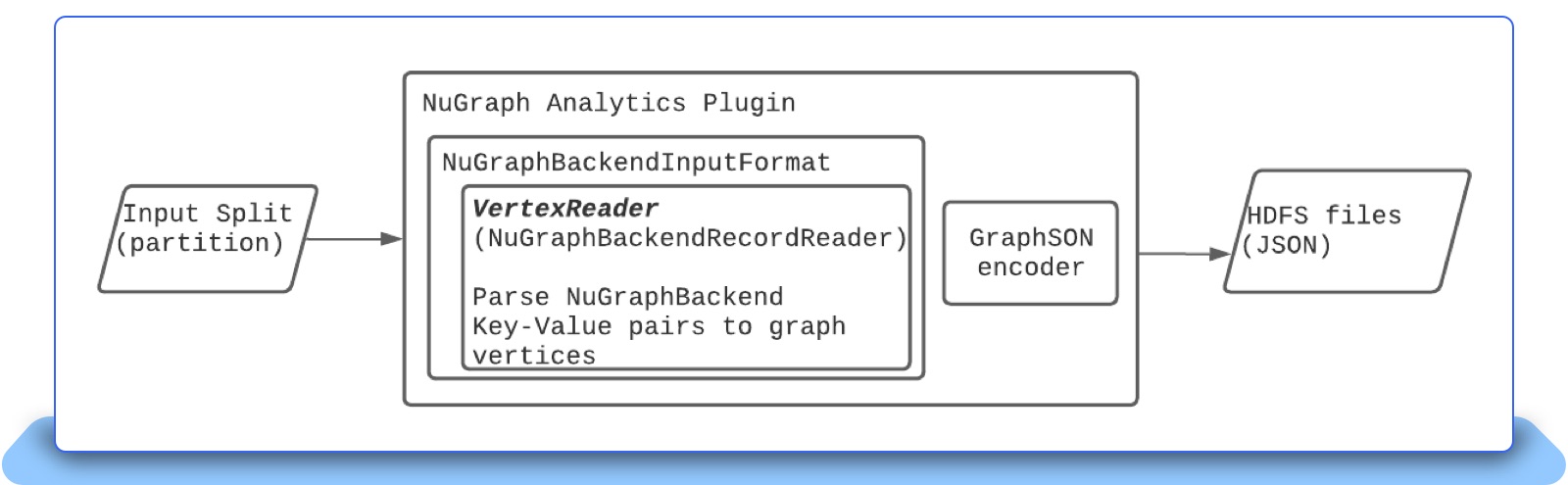
Figure 2: The NuGraph analytics plugin that converts NuGraphBackend partitions into Spark partitions, with Vertex Reader to parse Spark partitions into graph vertices.
Two new challenges arise related to the mapping of a NuGraphBackend partition to a Spark partition.
The NuGraph analytics plugin scans the backend store’s partition based on the partition mapping information exposed from the backend store. However, JanusGraph encodes the graph elements that involve vertex ID, vertex properties and edges as the ordered key-value pairs in a continuous key range, which then get saved into the backend store. Therefore, the backend store is not aware of such graph-level encoded information. As a result, when the scan result returns from the backend store to our NuGraph analytics plugin, the returned key ranges may split the same vertex that holds its vertex properties and edges into multiple different Spark partitions. Duplicated vertices could happen when parsing the key ranges by the Vertex Reader at the NuGraph analytics plugin. This issue is illustrated in Figure 3. The NuGraphBackend partition splits the Vertex ID1 and Vertex IDk into different spark partitions. Both the start and end point need to be aligned to the Spark partition boundary to guarantee a complete vertice-based key/value range.

Figure 3: Vertex-aware range alignment for the encoded Key/Value in NuGraph’s backend store.
The second challenge is due to the range alignment introduced above. If there is a vertex which has a large number of properties or edges, which is called “super node” [3], it is possible that the vertex can span across many continuous ranges, as shown in Figure 4. The NuGraph analytics plugin must guarantee that these continuous ranges are assigned to the same Spark partition for the Vertex Reader.

Figure 4: A super node vertex, which spans across three NuGraphBackend partitions in the backend store, P1, P2, and P3. These three partitions have to be assigned to the same Spark partition for the Vertex Reader.
The entire NuGraph analytics plugin solution is implemented as a JanusGraph analytics package over FoundationDB. The current analytics package is built upon the standard JanusGraph distribution that has analytics plugins to support Cassandra and HBase. In our analytics package, the main class extends the JanusGraph’s org.janusgraph.hadoop.formats.util.HadoopInputFormat, and implements the following two functions: getSplits() and createRecordReader().
The getSplits() generates a list of InputSplit by mapping the NuGraphBackend partitions to a Hadoop InputSplit, which addresses the challenges of mapping the NuGraphBackend partitions to Spark partitions, and aligning the unaligned Spark partitions. The createRecordReader() returns a RecordReader to iterate the NuGraphBackend partition, restart the iteration if timeout occurs, decode the NuGraphBackend partition, and build a Tinkerpop’s StarVertex, which represents a vertex and its associated properties and edges. Every StarVertex takes one line in JSON format. One HDFS file contains all StarVertex constructed from one Spark partition.
4. The ETL Pipeline
Figure 5 shows the end-to-end processing pipeline for the graph export. The DR cluster has the continuously synchronized update from the primary cluster. The NuGraph analytics plugin is developed as a Java library that gets loaded into Spark. Parallel key range scan over The NuGraphBackend partitions allows the raw key/value pairs to be retrieved, go through the vertex-aware range alignment, and then get converted into graph vertices (and their properties and edges) by the Vertex Reader. The vertices then get saved to HDFS in a JSON format, with one HDFS file representing one Spark partition. Once the whole graph gets stored to HDFS, other Spark jobs are launched for statistics and graph insights, such as the total vertex count and edge count.
The exported graph on HDFS is then accessed by the application-specific processing pipeline. For example, the exported graph can get converted into some HDFS data warehouse (DW) tables, ready for Spark-SQL processing.
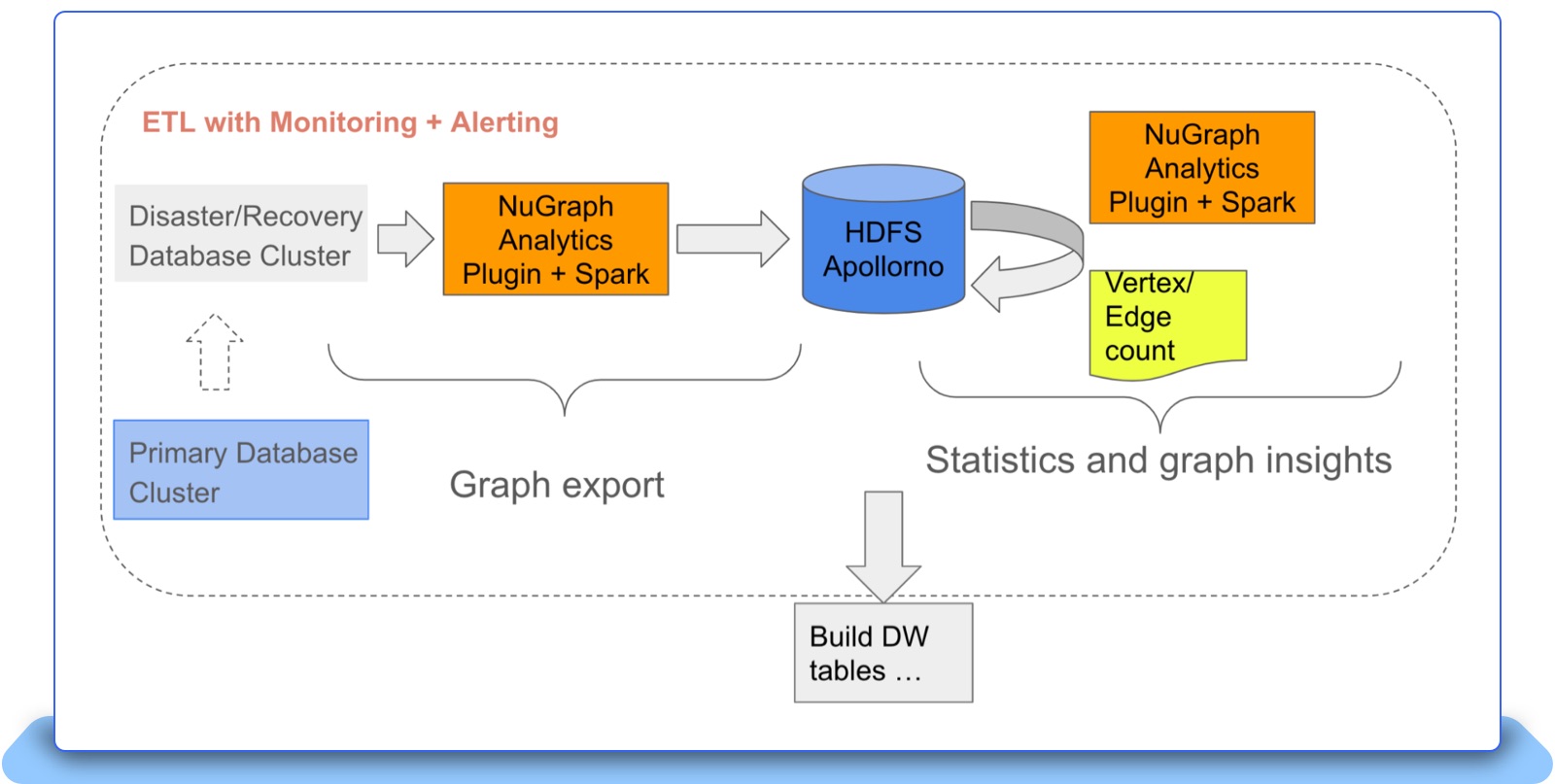
Figure 5: The end-to-end graph export pipeline.
5. JVM Memory Management
With the current JanusGraph standard distribution, the graph export from our NuGraph analytics plugin can be performed smoothly on the graphs that have up to hundreds of millions of vertices and edges. But when the graphs get to the scale of billions of vertices and edges, we start to encounter performance issues that are related to JVM memory management, including:
-
High GC overhead for exporting the graph from FoundationDB through Spark
-
Inefficient graph export processing in Tinkerpop
-
Out of memory (OOM) when running Gremlin analytical queries
-
High memory footprint for FoundationDB Java client library
We used Java Async profiler [6] and Eclipse Memory Analyzer Tool (MAT) [7] to troubleshoot the above performance issues.
In our production clusters, once these issues were resolved or mitigated, the overall graph export for the biggest graph with 15 billion vertices and over 24 billion edges was found to run smoothly, and the total export time was reduced to 3 hours from more than 5 hours.
5.1: High GC overhead for Exporting the Graph
The graph export job in Spark contains two stages. The first stage fully scans the backend storage, deserializes the key-value pairs to be a graph vertex object and cache the graph vertex object in Spark executor’s memory or disk if it is too big. The second stage serializes the graph vertex data to HDFS in JSON or GRYO [8] format.
During the experiment of exporting large graphs, Spark UI indicates that almost every executor’s GC overhead is higher than 10% (Figure 6). The flame graph captured by the JVM Async Profiler (Figure 7) also indicates the GC overhead is the main bottleneck. As a result, the graph export process is very slow.
In order to find the root cause of the high GC, we captured the JVM heap dump and analyzed it with the MAT tool. Figure 8 indicates that Java’s ConcurrentLinkedQueue holds quite a large number of Java objects. Considering the Guava cache, whose implementation uses ConcurrentLinkedQueue as the internal data cache and the class com.google.common.cache.LocalCache$Segment also shows up. All of those clues point to the conclusion that Google’s Guava cache is the root cause of this high GC overhead.

Figure 6: Spark Executors tab indicates high GC overhead.
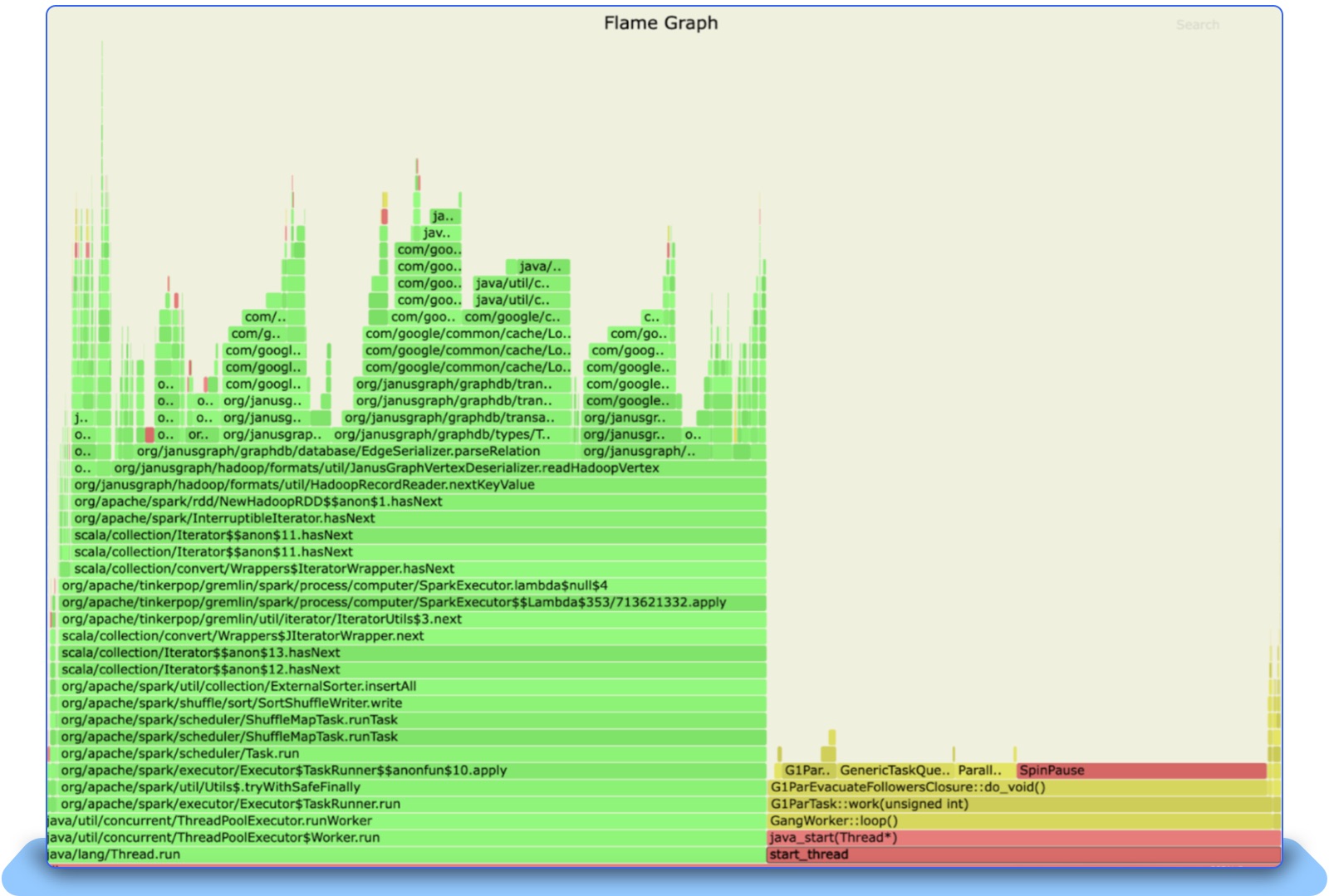
Figure 7: The Flame graph captured by the JVM Async profiler.

Figure 8: Java class histogram displayed by MAT
After reviewing the source code of Guava cache [9] and checking the known issues captured in Google Guava cache related Github [10], we came up with a fix: replace the Guava cache with another caching solution called Caffeine [11]. After the fix, the GC overhead disappears, and overall performance is improved by about 3X, on a synthetic graph that has 160 million vertices and 800 million edges.
We further tried to figure out under which circumstance the Guava cache related performance bug got triggered. Our Janusgraph code deep dive indicates the first stage of the graph export uses the Guava cache. In this stage, Spark executor calls HadoopInputFormat to process the partition. HadoopInputFormat registers a JanusGraphVertexDeserializer, which parses the Key-Value pairs, validates the data and decodes them to be a series of StarVertex objects. Every StarVertex is a single vertex together with its associated properties and edges. The JanusGraphVertexDeserializer maintains a VertexCache which maps a Long ID to an internal vertex object. Here the VertexCache only caches the Long ID mapping to a graph schema vertex – for example, property key vertex, label vertex, and edge vertex. Such schema definition objects are referenced in the graph as deserialized objects, and thus shared among all graph objects. Figure 9 is an example displaying what is saved in the VertexCache.
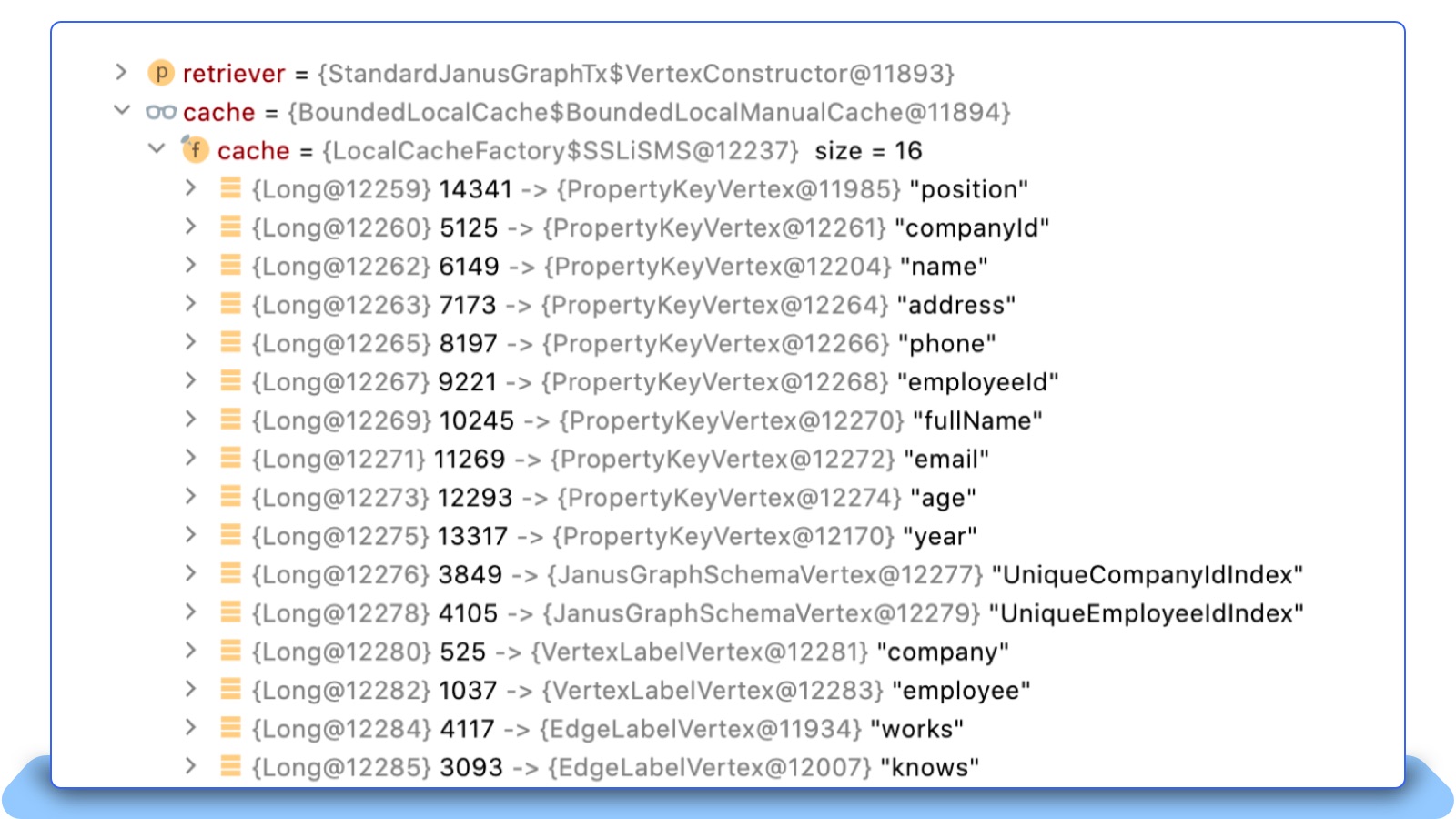
Figure 9: VertexCache contains 16 entries, each of which is a schema definition object
In Janusgraph 0.6.1, the Guava cache serves as a Least Recently Use (LRU) cache in the implementation of VertexCache. For a big graph with 160 million vertices and 800 million edges, this VertexCache only has 16 entries, but the getIfPresent() function implemented by Guava cache is invoked 3,018,666,935 times. For a typical LRU cache, the “get” operation also triggers a “put” operation to the internal cache. In a high concurrent and busy Spark executor, the huge VertexCache “get” operation caused a lot of new Java objects to be created and “put” to the LRU cache.As a result, it triggers the known issue in Guava cache [10]. In contrast, Caffeine cache internally used a ring-buffer to save the latest access item and thus fix this issue. That explains why GC overhead disappears after applying Caffeine cache. The Janusgraph community has already adopted our fix [12].
5.2: Inefficient Graph Export Implementation in TinkerPop
In Tinkerpop, the graph export is supported by the following Gremlin query:
|
graph.compute(SparkGraphComputer).program(CloneVertexProgram.build().create()).submit().get() |
Tinkerpop’s spark component runs a VertexProgram [13] in the Bulk Synchronous Parallel (BSP) [14] fashion, which is a general computational framework for graph computing. Tinkerpop’s implementation relies on Spark’s broadcast variable [15] and data-frame joining. Note that data-frame joining is an expensive operation, requiring a huge data exchange from the remote nodes and a lot of network traffic, for a big graph.
The general VertexProgram can be optimized, which is used for graph export and based on CloneVertexProgram. Tinkerpop’s SparkGraphComputer [16] can be easily optimized to remove unnecessary shuffles when the CloneVertexProgram is used for graph export. The PR [17] from our particular improvement provides optimization to this operation and reduces the operation from three stages to two stages, which gives 1.4X ~ 1.5X performance benefit.
5.3: Out-of-Memory in Gremlin Analytics Queries
Following what is described in Section 5.2, Tinkerpop’s SparkGraphComputer leverages Spark’s broadcast variable to implement message passing, and saves the result into the broadcast variable. Generally, that is acceptable. But for a large graph, this solution leads to high memory pressure. The broadcast variable which is saved in Tinkerpop’s ObjectWritable may cause OOM. The source code ObjectWriable.java [18] has a function toString() to display its variable’s content. In some experiments, the content can be huge, as shown in Figure 10.
The long string text is, generally, unimportant, and only for UI displaying. We optimized this function to reduce to toString()’s returned value if it is a Java Collection or Map, thus avoiding the potential of generating a large array of long integers. The PR associated with this particular optimization [19] has been accepted by the Tinkerpop community.
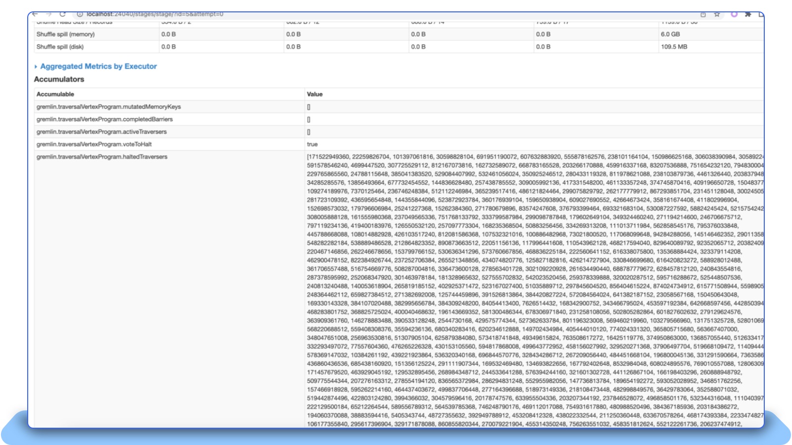
Figure 10: SparkUI’s Stages tab indicates that an Accumulable contains a large array of long integer values.
6. Performance Measurement
We provide some measurement results on the graphs exported from our production clusters. The time spent on graph export depends on the graph size. The following table shows the export time and HDFS file size along with the graph size. The Account-Linking graph and the Buyer-Follow-Seller graph are two different graphs hosted in our production clusters. LDBC benchmark [20] is a popular benchmark used in the graph database industry.

Table 1: The graph export time for different graphs along with their graph sizes and HDFS file sizes.
7. Graph Structure Analysis
Given an exported graph, besides the graph size reporting in terms of vertex count and edge count, we can do various useful graph structure based analyses. In terms of graph quality assurance, we would like to the answer on: (1) does the graph have some vertices (called ghost vertices) that have no incoming and outgoing edges, and (2) does the graph have some vertices that have the number of incoming or outgoing edges exceeding some thresholds (for example, over one million). The detection of such abnormal vertices can reveal data loading issues or data preparation issues from the application.
Often, the transactional query latency can be controlled by pruning the incoming and outgoing edges of each vertex, so that each vertex has the edge count to be within a threshold, say, 100. An analysis tool can identify the candidate vertices that need to be pruned across the entire graph. Such candidate vertices can be loaded by another tool like GraphLoad [21] that invokes a transactional query on each candidate vertex to query the actual edges and then remove the excessive edges.
Graphs that capture real-world relationships typically follow a power-law [22] distribution in terms of the outgoing and incoming edges. For our buyer-follow-seller graph, which is like a social networking graph, Figure 13 shows that such a buyer-follow-seller relationship does form a power-law distribution. The x-axis is the vertex degree, which is defined as the sum of the incoming and outgoing edges, and the y-axis is the total vertex count that has the corresponding vertex degree. Both x-axis and y-axis are shown a logarithmic scale. Figure 13 indicates that most of the vertice have very small degrees. For example, the number of vertices that have degree of 10 is 344,599, and the number of the vertices that have degree of 100 is 6,058, and only 96 vertices have the degree of 1000.
A power law distribution has the form of Y = k X-ɑ. X and Y are variables of interest, α is the law’s exponent, k is a constant. By taking the logarithmic operation on both sizes of the equation, we can have the following expression:
log(Y) = log(k) -αlog(X)
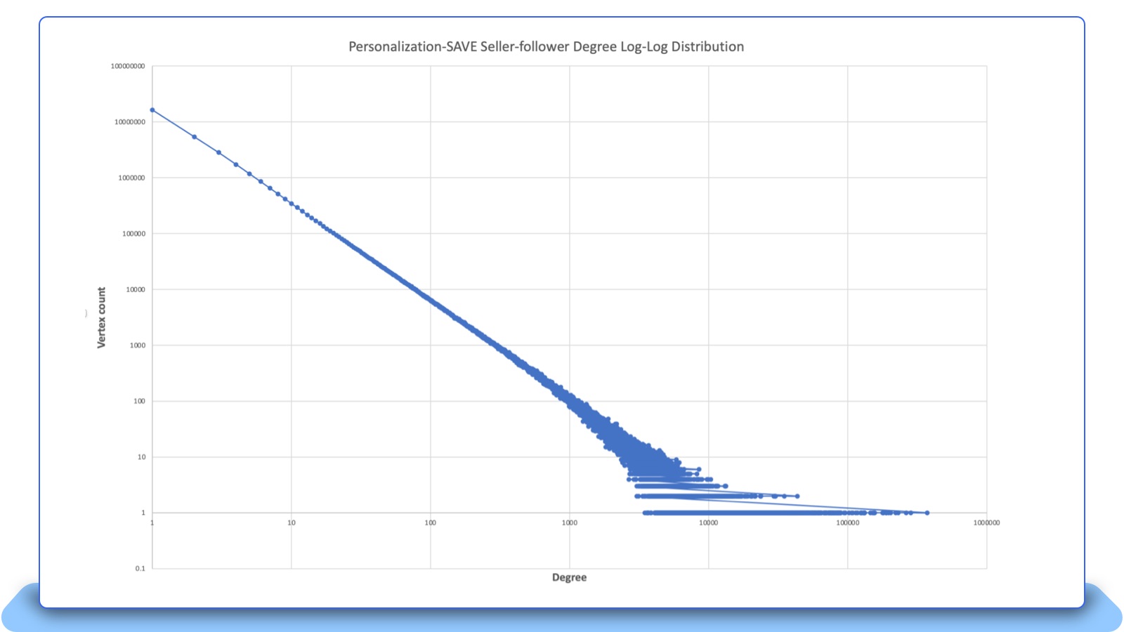
Figure 13: The power-law distribution for the buyer-follow-seller graph.
8. Conclusions
To support graph analytics, we have developed an analytics plugin over the JanusGraph standard distribution to support graph export over the NuGraph transactional backend store, which currently is based on FoundationDB. This graph export utility performs a parallel full scan against the backend store and produces the exported graph in HDFS. The graph export utility has been into production since early 2023 and able to export the graphs with billions of vertices and edges, including the graph that has over 15 billion vertices and 24 billion edges. We have developed various techniques and improvements to accommodate such large graphs in production, including separation of offline graph export from online transactional query traffic, handling of super nodes in graphs, and to address many inefficient JVM memory management issues that manifest themselves only when processing billions of vertices and edges to support eBay’s millions online transactions.
References
[1] JanusGraph Introduction, https://docs.janusgraph.org/
[2] FoundationDB 7.2, https://apple.github.io/foundationdb/
[3] A Solution to the Supernode Problem https://www.datastax.com/blog/solution-supernode-problem
[4] Gremlin Query Language https://tinkerpop.apache.org/gremlin.html
[5] Welcome to Nebula Algorithm https://github.com/vesoft-inc/nebula-algorithm
[6] Async-profiler https://github.com/async-profiler/async-profiler
[7] Memory Analyzer (MAT) https://www.eclipse.org/mat/
[8] GRYO https://tinkerpop.apache.org/docs/current/reference/#gryo
[9] https://github.com/google/guava/blob/master/guava/src/com/google/common/cache/LocalCache.java
[10] Guava LocalCache recencyQueue is 223M entries dominating 5.3GB of heap
https://github.com/google/guava/issues/2408
[11] Caffeine Cache https://github.com/ben-manes/caffeine
[12] Replace Guava cache with Caffeine cache https://github.com/JanusGraph/janusgraph/pull/3188
[13] Vertex program https://tinkerpop.apache.org/docs/current/reference/#vertexprogram
[14] Bulk synchronous parallel https://en.wikipedia.org/wiki/Bulk_synchronous_parallel
[15] Spark broadcast variable https://spark.apache.org/docs/2.2.0/rdd-programming-guide.html#broadcast-variables
[17] Optimize CloneVertexProgram through SparkGraphComputer https://github.com/apache/tinkerpop/pull/1885
[19] Shrink the content of ObjectWritable.toString() https://github.com/apache/tinkerpop/pull/2050
[20] https://ldbcouncil.org/ldbc_snb_docs/ldbc-snb-specification.pdf
[21] GraphLoad: A Framework to Load and Update Over Ten-Billion-Vertex Graphs with Performance and Consistency, by T. Schweiger, H. Nguyen, J. Li, L. Hu and S. Gopalsamy, 2021. https://innovation.ebayinc.com/tech/engineering/graphload-a-framework-to-load-and-update-over-ten-billion-vertex-graphs-with-performance-and-consistency/